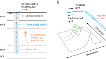
To unravel fault zone properties, high-resolution imaging and probing are pivotal. Here we present a comprehensive study utilizing Distributed Dynamic Strain Sensing of a 3D array of optical fiber with a surface-to-depth installation, traversing an active fault zone at depth, combined with a geological analysis of drilled cores. We identify an asymmetric fault zone with a narrow fault core, exhibiting a notable amplification in strain rate across a broad-band frequency range, which is attributed to the presence of weak gouge material within a much stronger host rock. This feature heightens responsiveness of the weak fault zone with low rigidity to ground motion, and intensifies strain from both nearby and remote seismic events. We demonstrate that optical fiber facilitates long-term monitoring of ground motion amplification with high spatial resolution, thus indicating where strain and deformation accumulate through repeating ruptures. This progress is pivotal to the understanding of the role of low rigidity and changes thereof within fault gouge material.
Earthquakes occur along faults spanning ~1–100 s km with varying thicknesses of ~0.01–10 s meters, exhibiting material properties distinct to the enveloping rock mass 1 . To unravel fault zone properties, high-resolution imaging and probing are pivotal for advancing insights into rupture dynamics, earthquake source properties 2,3 , ground motion 4 and the seismic cycle 3 . This is particularly crucial for assessing the impact of destructive earthquakes, often stemming from blind faults and multiple-fault segments in fault systems 5,6,7 . Despite its significance, technological limitations and logistical challenges are detrimental in developing instruments for recording seismic data to accurately capture not only the fault system but also structures within fault zones, where subtle movements and complexities demand a higher level of precision. The growing availability of distributed fiber optic sensing facilitates ground-motion assessment at intervals of a few meters along kilometers of cable, delivering unparalleled subsurface structural resolution 8,9,10,11,12 , exceeding conventional dense arrays 13,14 . A novel approach entails installing fiber in a borehole crossing a seismogenic fault, enabling intensive and continuous fault zone measurements in a natural setting.
Logistical challenges, such as deploying sensors in remote or geologically complex fault regions, or urban areas with restricted access, limit comprehensive data acquisition. In earthquake-prone Taiwan, Hualien City experienced a damaging MW 6.4 earthquake in 2018 15 . The event struck close to the shore at a depth of ~6.3 km, inducing primary surface ruptures along the inland Milun fault 16 (Fig. 1a, b), coupled with left-lateral high-angle reverse faulting dipping eastward 17,18 . The spatial concurrence of these surface ruptures with those from the 1951 MW 7.2 Hualien earthquake 19,20,21 (Fig. 1a) underscores the Milun fault’s pivotal role as a principal seismogenic fault within the region. The Milun fault in Hualien City is proximal to the Ryukyu subduction zone, a tectonic plate boundary between the Eurasian plate and the Philippine Sea plate (Fig. 1a), and offers an opportunity for an investigation of a dynamically active fault zone, with frequent slip, by deploying high-resolution distributed fiber optic sensing crossing the fault at depth and the surface. Owing to its urban context, the fault’s accessibility facilitates an integrated study involving borehole drill coring and the permanent deployment of a 3D optical fiber sensing array (Fig. 1c). The setup for Distributed Dynamic Strain Sensing (DDSS; under its more generic term is also known as Distributed Acoustic Sensing [DAS]) at the Milun fault consists of the sensor gauging the fiber’s response to external forces by measuring strain rate over a gauge length of 10 m at 4 m intervals throughout the entire fiber with a total length of 6380 m and a sampling rate of 1000 Hz. In addition, we benefit from the borehole’s drill core as a geological archive, allowing a comprehensive analysis of core samples alongside detailed fiber measurements, providing direct evidence of fault zone behavior with depth.
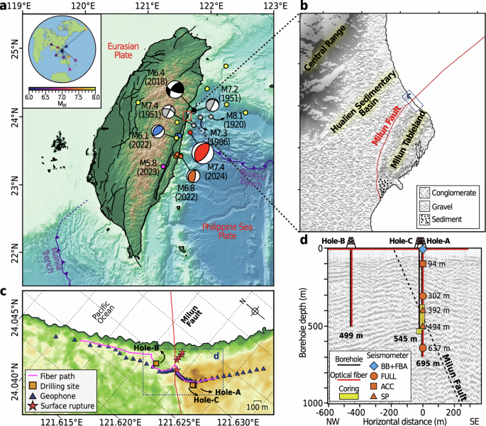
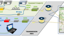
Suitable borehole locations were identified through detailed seismic surveys (Fig S1), identifying two sites on the hanging wall (Hole-A, Hole-C) and one on the footwall (Hole-B) of the surface rupture zone (Fig. 1c). Drilling activities were conducted from January 2022 until October 2022 reaching depths of 695 m, 499 m, and 545 m for Hole-A, Hole-B, and Hole-C, respectively (Fig. 1d). We designated Hole-A (January 2022) and Hole-B (June 2022) primarily for optical fiber installation, while Hole-C (located 21 m apart from Hole A) is an auxiliary borehole for fluid and gas monitoring. Seismic survey profiles at Hole-A identified a potentially major fault intersecting the borehole at approximately ~500 m depth (Fig. 1d, and Supplementary Fig. 1) and dipping east at ~70 o . Figure 1c-d show the array’s loop configuration starting with a descent from the surface to a depth of 700 m (Hole-A) along the hanging wall of the Milun fault, crossing the fault at depth before resurfacing, and extending along the surface to intersect the surface fault rupture zone. We also use existing fiber infrastructure from ChungHua Telecommunication (CHT) company in the densely populated town area near the Milun fault to explore the feasibility of commercial fiber for seismic analysis and to connect our fiber between the two borehole sites. The loop continues to the second borehole (Hole-B) down to a depth of 500 m on the footwall side of the Milun fault. The loop extends northward of Hole-B and eastward from Hole-A (Fig. 1c). The fiber is externally affixed to the borehole casing and cemented for optimal coupling with the rock mass. This configuration enables a comparison between fault zone identification using the specialized installed fiber and surface rupture signatures detected with commercial fiber 10 . While all boreholes underwent logging, coring was limited to Hole-A and neighboring Hole-C (without fiber), as we expected to encounter the fault zone there (Fig. 1d). After the successful installation of the optical fiber, we deployed a vertical seismic array in Hole-A comprising of five borehole seismometers (Fig. 1d), facilitating direct comparison of the fiber records with these from conventional borehole seismometers and ensuring reliable amplitude measurements throughout the optical fiber system in the borehole 9 ..
Prior observations of strain amplification in weak zones 9,14,22 with optical fiber have been reported, however, our concurrent examination of coring, logging, and fiber sensing allows for a comprehensive analysis of core samples in conjunction with detailed fiber measurements. This approach provides detailed insights into fault zone behavior at depth, free from surface interference, and is a reliable benchmark for utilizing optical fiber as a sensing tool for faults at depth. We identify an asymmetric narrow fault core that exhibits significant strain rate amplification, observed across a broad frequency band. This amplification results from weak gouge material surrounded by a stronger host rock. By leveraging the high spatial resolution and long-term monitoring capabilities of optical fiber, we propose that this asymmetric broad-band strain-rate amplification could serve as a detailed indicator for fault delineation, particularly in narrow fault zones only a couple of meters wide. Recognizing the role of low rigidity in fault gouge material identified through DDSS contributes valuable insights into fault zone behavior, especially with the long-term monitoring capability of DDSS. Moreover, the subsurface site response observed through borehole optical fiber captures further detailed fault-related information.
In addition to DDSS recording, Distributed Temperature Sensing (DTS) measurements were utilized after the installation of borehole optical fiber during cementing to directly monitor the success of the cementing process, ensuring optimal fiber-wellbore coupling necessary for the reliability and effectiveness of the distributed optical fiber system in the borehole. The uniform and homogeneous temperature profile observed in DTS monitoring 23 (Supplementary Fig. 2) ensures minimal variability in DDSS records with depth. Utilizing duplicate downward and upward DDSS channels along the borehole, we examined DDSS waveform fidelity with a spatial resolution of 4 m by root-mean-square amplitude (rms) ratios and cross-correlation analysis between data from different channels at similar depth. The rms ratios average is approximately 1 with a standard deviation of 0.02, indicating around 2% variability in DDSS amplitudes along all borehole channels (Fig. 2a). Moreover, all zero-lag cross-correlation coefficients (c.c.) of DDSS waveform pairs from borehole channels exceed 0.981, suggesting nearly identical waveform phases 24 . The low variability in the rms amplitude ratios and very high signal cross-correlation coefficients suggest that our borehole DDSS observations are free from any signal fading.
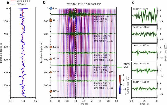
We show that the concurrent installation of optical fiber with borehole seismometers enables a comprehensive examination of seismic quality, leveraging state-of-the-art technologies as a complement to previous studies 8,9,10 employing surface stations. The comparison of DDSS records to seismometer-array derived strain-rates 25,26,27 from a local ML 5.3 earthquake (Fig. 1a) reveals high correlation at various depths (Fig. 2b, c.c. > 0.9), with rms ratios within 30% difference range for peak values between 1.130 and 1.623 of the selected time windows (Figs. 2b-c). Comparable rms ratios and high cross-correlation coefficients with depth indicate reliable fiber-wellbore coupling, despite differences in the analysis of strain rates derived from a seismometer array and DDSS, regarding the instrument type (borehole seismometer vs. DDSS) and the assumptions regarding media homogeneity-related to sensor spacing (DDSS: 10 m, seismometers: at least 100 m).
Recognizing fault cores within fault zones is crucial for unveiling the intricate fault zone architecture 28,29,30,31 . Core sampling from Hole-A spanned 361.8 m to 522.9 m but halted due to coring complications. We obtained core samples from Hole-C from depths between 507.9 m and 543.3 m (Fig. 1d). Supplementary Fig. 3 shows the geophysical logs for Hole-A, and Supplementary Fig. 4 shows the comparison of geophysical logs (gamma, and resistivity) and core characteristics from Hole-A (514.10m-514.25 m, 516.70 m, 522.15 m) and Hole-C (516.27m-516.42 m, 518.5 m, 526.55 m). The consistency in geophysical logs and identified core characteristics, despite the spatial separation of 21 m, suggests that the core of Hole-C is representative for Hole-A below a depth of 522.90 m. Thus, the borehole core samples obtained from 361.8 m to 522.9 m in Hole-A and from 507.9 m to 543.3 m in Hole C can be considered as continuous cores that penetrate the Milun fault. Given their lithological coherence, proximity, and complemented by logging data, subsequent descriptions amalgamate both cores as a single unit. Between ~490 m and 540 m, the cores unveiled distinct physical, lithological, and structural characteristics of the fault zone, sharply contrasting with the conglomerate composition of the surrounding hanging wall and footwall. The specific interval between 491.05 m and 540 is denoted as the Milun Fault Zone (MFZ), which is enclosed by Milun conglomerate on the hanging wall and footwall (Figs. 3a, and b). The conglomerate is characterized by rounded to sub-angular, gravel-sized metamorphic clasts embedded within a matrix featuring varying proportions of sand and clay. In contrast, the MFZ displays interconnected zones with variable widths of clay within spotted schist (Hole-A: 491.05 m to 516.80 m, Hole-C: 517.78 m), non-cohesive serpentinite (Hole-A: 516.80 m to 520.45 m, Hole-C: 517.78 m to 525.20 m), and foliated gray and black gouges (Hole-A: 520.45 m to 522.90 m, Hole-C: 525.20 m to 540.30 m). All reported depths related to the cores are measured with respect to the boreholes. Mineralogical phases of the materials of each rock shown in Fig. 3a were determined by in-situ synchrotron X-ray diffraction analyses (Supplementary Fig. 5). The analyses were operated with a beam size of 150 μm in diameter 32,33 . Spotted schists and serpentinite constitute the lithological assemblage of the Yuli belt, a metamorphosed mélange from the middle-late Miocene, located at the eastern limb of Taiwan’s orogenic belt 34 . This assemblage, characterized by anastomosing clay-rich veins and noncohesive attributes, signifies long-term fluid-rock interaction and substantial water circulation involving the MFZ. Notably, the depth range of 520.45 m to 540.30 m corresponds to the fault core, distinctly marked by the foliated gray and black gouge (Fig. 3a).
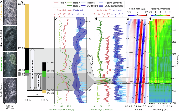
The borehole core revealed an asymmetric fault architecture between 490 m and 540 m. A distinctive fault damage zone surrounds the gouge-bearing fault core on the hanging wall, while no evident damage zone was identified on the footwall between depths 520 m − 540 m (Fig. 3b). The projection of this fault damage zone depth in Hole-A to the surface rupture of the fault 21 aligns with the 70 o east dip of the Milun fault identified in the seismic profile.
With the comprehensive analysis of core samples and geophysical logs, we derive a P-wave velocity profile (VP) by analyzing cross-correlations of borehole DDSS records from seven local earthquakes (Fig. 1a, Supplementary Table 1, Fig. 3e, and Supplementary Fig. 6a-b). To extract the arrival time differences between channels, we employed an adaptive stacking method 35 on the windowed P-wave arrivals, filtered between 1.2 to 5 Hz. Given the spectral bandwidth, the P-wave velocity profile uses a channel spacing of 40 meters (= 10 channels) 36 . This analysis involves surface reflection elimination (Supplementary Fig. 7), and incident and refraction angle correction (Supplementary Fig. 8) by using pseudo-bending ray-tracing 37 with a 3-D velocity model 38 for travel-time correction to the phases. Since the incident angles of P-wave signals from the analyzed earthquakes are sub-vertical, i.e., sub-parallel to the fiber cable, the effect of directional sensitivity is negligible and is ignored for our phase analysis. The adaptive cross-correlation yields precise travel time differences forming the velocity profile (Supplementary Fig. 6c-d). With minimal variability in the events, the DDSS cross-correlation-based VP estimate aligns overall with the logging-based VP, which was sampled every centimeter and averaged per meter (Fig. 3c and d). The VP ranges within 2–3 km/s, except for a notable dip to ~1.5 km/s between 510 m and 550 m, i.e., within the MFZ. In alignment with noticeable lithological variations observed in the core samples, we discern distinctive traits in the geophysical borehole logs, encompassing gamma ray, resistivity, and low compressional wave velocity (VP). The gamma-ray and resistivity logs show clear signatures within the MFZ (Fig. 3c and d). In addition, notable variations in phase shift and amplitude in the MFZ, particularly in the lower portion linked to the fault core (Fig. 3e). Figure 3f shows the average amplitude spectrum of these local earthquakes, normalized to amplitudes in the deepest borehole section. In the MFZ depth range, P-wave amplitude spectra are 2-3 times larger at all frequencies across all events (Fig. 3f) compared to spectra of the wave field below the MFZ. This suggests an influence of fault zone materials on the seismic strain-field amplitudes. Analogous, albeit weaker, amplification patterns at depths ~310 m-330 m and ~160 m-180 m suggest localized features with weak material in the overlying conglomerate layer or other lithological contacts. These amplification signatures demonstrate the capability of optical fiber sensing to image borehole structures 22 .
To further unveil insights into both subsurface fault zones and their corresponding surface rupture zones from optical fiber, we analyzed DDSS records of two well recorded local earthquake sequences, related to the MW 6.8 event on March 22, 2022, and the MW 6.1 on June 20, 2022 (Fig. 1a, Supplementary Table 2). Four earthquakes of the March sequence and three earthquakes of the June sequence are selected, ranging from MW 3.8 to 6.8. We identify P-wave windows, determine peak strain rates for each borehole channel, and normalized w.r.t. the mean of the channels in the bottommost 100 m of the borehole (Supplementary Fig. 10a). This normalization, relative to the bottommost 100 m, is in line with the consistent phases of the strain wavefield below 650 m (Fig. 4c), corresponding to the depth where the footwall acts as the host rock as seen in the retrieved fault core (Fig. 3a).
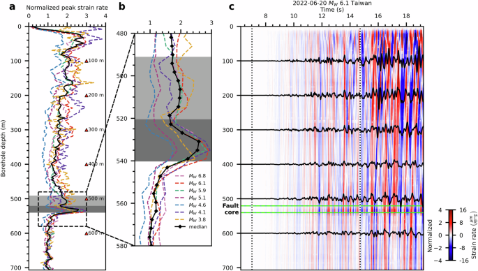
Figure 4a shows the normalized peak strain rates ranging from 1.5-3 with a median of 2.5 (cf. Fig. 3f). Despite some variation, all events evidently have decreasing amplitudes with depth and display amplification in the fault zone. The MFZ is marked by a distinct amplitude spike at the fault core’s lower boundary (Fig. 4b). We note an overall asymmetrical amplification pattern, which correlates with the locations of the lithological phases identified in the retrieved cores (Fig. 3b), the geophysical logs and cross-correlation analysis (Fig. 3c and d). The strain-rate signal is amplified within the fault zone at all times, as exemplified by the P-waves of the June 2022 M 6.1 earthquake (Fig. 4c). In contrast, a similar fault-zone-related amplification pattern is absent in Hole-B, and peak strain rates from the same event in Hole-B exhibit attenuation with depth only (Supplementary Fig. 10).
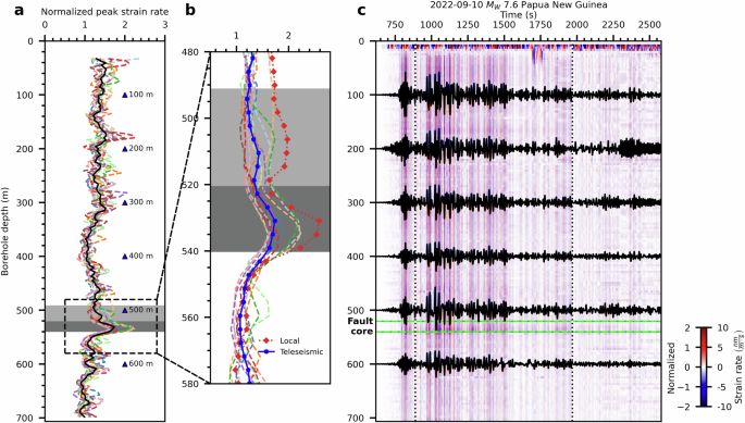
The interaction of seismic waves with the MFZ extends beyond local seismic activity. We recorded multiple teleseismic earthquakes with MW > 6 between May and October 2022 (Fig. 1a, Supplementary Table 3) with high signal-to-noise ratios. Considering the good azimuthal coverage of our array, we selected a total of eleven teleseismic earthquakes. Given the vertical alignment of the borehole fiber, records of teleseismic events will be dominated by low-frequency (W 7.6 Papua New Guinea earthquake. For the amplitude comparison, the median of the absolute strain rate is computed for each channel within the time windows, and these averages are normalized by the median of the averages of the 10 deepest channels (spanning ~40 m). Thus, the amplifications are relative to the strain rate amplitudes at the bottom of the borehole. We obtain normalized absolute strain rate amplification in the range of 1.5-2.2 with a median of about 1.6 in the MFZ (Figs. 5a and b). The amplification is slightly less than that for the local events, but the asymmetric pattern remains (cf. Figure 4a and b). Despite the differences between local and teleseismic events (subvertical vs. horizontal incidence, high vs. low frequency content, body vs. surface waves), showing this strain-rate amplification is not only present across the broad-band range of wave frequencies, but also implies a direct correlation between observed strain-rate signals and material properties of the fault zone and its host rock. This effect of material properties also links the amplitude changes with the corresponding changes in VP from the cross-correlation analysis and logging (Fig. 3d).
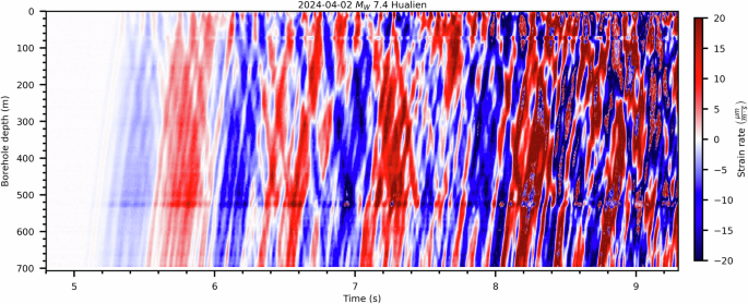
On April 2, 2024, Hulien City was hit by a MW 7.4 earthquake, approximately 20 km from the DDSS array, with a peak ground acceleration of about 0.32 m/s 2 at the nearest strong-motion station. The DDSS record of this earthquake is shown in Fig. 6. Although the signal saturated a few seconds after initial arrivals, the recording system performed adequately during strong shaking. Similar to the smaller local events (Fig. 4c) and the teleseismic events (Fig. 5c), the waveforms (Fig. 6) exhibit noticeable amplification in the depth range of the MFZ from the first motion on.
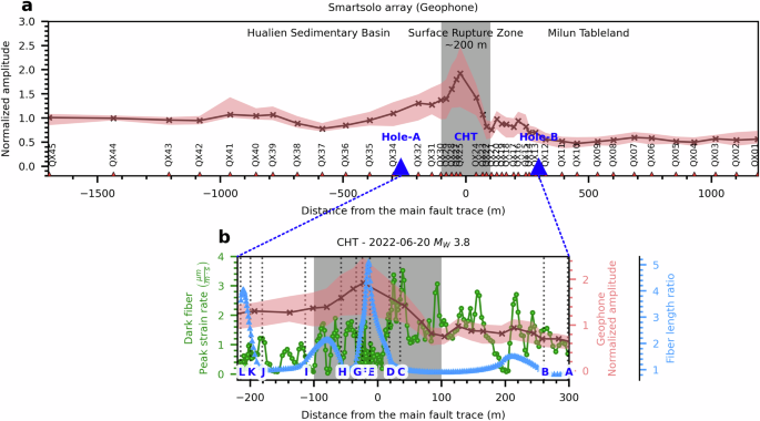
Based on the fault core characteristics at depth we investigated whether the seismic wavefield could reveal the corresponding surface rupture zone through commercial fiber, which has been shown to be effective 8,9 . While commercial fiber might not inherently meet seismological requirements, we thus supplemented the commercial fiber analysis by integrating a previously deployed (May 2021) collocated dense geophone (Smartsolo) array (Fig. 1c, and Supplementary Fig. 11), with sensors installed every 100 m, and every 25 m near the surface rupture zone 39,40 caused by the 2018 Hualien earthquake. We selected 42 earthquakes recorded by geophone in May 2021 (Supplementary Fig. 12). We obtained the peak ground velocities of the vertical component filtered between 1.5 and 10 Hz, normalized to the northernmost stations along the array. Figure 6a displays the distribution of normalized median peak ground velocity of the vertical component within the array. The geophone array outlines a 200-meter amplification zone, coinciding with the 2018 earthquake’s surface rupture zone 39,40,41 . This amplification zone experiences a rapid drop on the southeast side, corresponding to the highland near Hole-A, rather than the sediment basin to the northwest of the profile near Hole-B (Fig. 1b).
In April 2022, a dark fiber 200-m-segment from Chunghua Telecom (CHT) was spliced with our fiber to combine Hole-A and Hole-B to form a 3D optical fiber array crossing the Milun fault. Supplementary Fig. 11a outlines the route of the CHT section, primarily following storm drains. The telecom fiber serves as a branch line from the existing optical fibertrunk. DDSS channels of the CHT section were located by tap tests between Hole-A and -B along the storm drain inlets (A-L, Supplementary Fig. 11b). Peak strain-rates for the June 2022 event sequence (MW 3.8) along the CHT section reveal similarities in relative amplitudes for DDSS channels north of the CHT section. However, the amplification pattern is disrupted with almost vanishing strain rates near storm drain inlets, a feature also visible for other events (Supplementary Fig. 13). The peak strain rate amplitudes vary along the CHT fiber, with lowest amplitudes corresponding to storm drain access points, which probably host spare fiber for maintenance purposes. We identify these spare fiber areas by comparing the fiber length to ground distance (Fig. 7b). Unfortunately, the highest ratio of fiber length to ground distance coincides with the location of the center of the surface rupture zone and where the highest amplitudes were recorded on the geophones (Fig. 7a). As such, the dark fiber can only partially capture the amplification pattern across the surface rupture zone, raising concerns about the viability of using commercial telecommunication fiber for seismic studies. Our observation implies the possibility of detecting surface rupture zones through amplified ground motion 9,10,11,12,13 using commercial fiber, but are limited by their setup, especially if branch sections of the commercial fiber network are utilized.
DDSS records revealed broad-band amplification of strain rate in the weak zone, and significantly within the MFZ, with distinct asymmetric features on the hanging wall and footwall. This asymmetry is also apparent in geophysical logs, particularly in gamma-ray counts (Fig. 3c) and to a lesser degree in logging VP and resistivity due to technical challenges of the borehole measurements. The asymmetry of the fault zone is also less discernible from the cross-correlation analysis of the DDSS data, where we used a 40 m moving window to ensure frequency stability. Neither logging nor cross-correlation reach a similar level of spatial resolution when directly recording strain by DDSS continuously, which forms the basis for identifying the fault zone and its asymmetry from amplitude variations.
The high spatial resolution of the vertical optical fiber captures resonance effects 42,43 appearing as increased amplification at certain frequencies in addition to the already amplified signals in the fault zone, e.g. the prominent amplification at 1.2 Hz reaching from the fault zone to the surface (Fig. 3f). The resonance effect is prominent in the structure, particularly above the fault zone but the associated signal amplification is not linked directly to the strain amplification resulting from changes in material properties. Both resonance and fault zone material effects appear independently and can exhibit constructive interference at certain frequencies. Overall, the strain amplification within the fault zone relative to the host rock at the bottom 100 m range between 1.6-3.0 (Figs. 4b, 5b), this variation might be influenced by incidence angle, and wave polarization (e.g. from body waves vs. surface waves) in the fault zone. These fault-zone-related strain amplifications are profound in all observations 44 . While the fault-zone-related amplification is more pronounced for local earthquakes than teleseismic events (Figs. 4a, 5a), both event types exhibit an asymmetric pattern, indicative of the fault zone architecture confirmed from the borehole core.
To validate our hypothesis of observed strain rate amplitude variations linked to material properties within the fault zone, we conduct a finite-difference simulation for approximation of the elastic wave equation 45 . We construct a 2D profile, perpendicular to the trace of the Milun fault, including the borehole location. Our simulation entails a vertically incident P-wave within a heterogeneous elastic medium, featuring an inclined planar fault zone with two embedded layers (as observed in the core, one for the fault core as fault gouge at the bottom, one for the damage zone as spotted schist on top) (Fig. 8a). To account for uncertainties in material properties 46,47 , a suite of models is run (Supplementary Table 4).
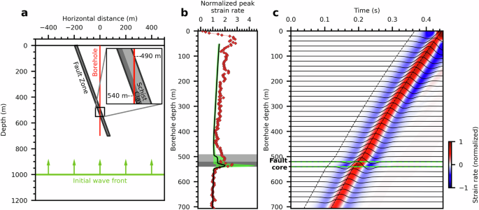
The simulated waveforms (example in Fig. 8c) are similarly processed as the DDSS records to determine the peak strain rate profile with depth and the median and range from all simulated amplitude ratios are computed. The amplification pattern of peak strain rates (ranged from 1.5-4.0) in the simulations along the borehole corroborates our observations (Fig. 8b). Notably, amplification is asymmetric and occurs near the fault zone, where the fault core interfaces with the host rock. The simulations show a large amplification variability given the sensitivity of strain rate to material properties (Fig. 8b), with our observations falling within this range. The strain rate contrasts shown by the simulations demonstrate the potential of DDSS to locate material contacts. With its high spatial resolution, DDSS can uncover even details within such intricate structures—insights hitherto accessible only through direct core sampling or core logging. Moreover, DDSS offers the additional advantage of precise, long-term monitoring of the temporal evolution of the fault.
The identification of fine-scaled fault zone features with geophones or borehole seismometers alone without costly logging and coring only became feasible with DDSS. Furthermore, DDSS facilitates continuous monitoring. Precision in fiber installation also pertains to coupling, as variations in fiber cable coupling, common in commercial fiber installations, will inadvertently affect signal quality and reduce the potential to identify fine-scaled signatures, e.g., related to faults or surface ruptures. Notably, changes in strain (rate) directly correspond to variations in the elastic moduli 48 . In as much as the fault zone’s asymmetric nature places the fault gouge in direct contact with the conglomerate host rock—creating a sharp and intense material property gradient—result in a significant change of strain (rate) amplitudes. Both data and models localize the highest strain rate amplification at the fault core’s lower side, where the fault gouge directly interfaces with the conglomerate host rock. This observation aligns with the substantial difference between the elastic moduli of the clay-bearing gouge and the conglomerate. The interrogator samples every 4 m with a gauge length of 10 m, and since the fault zone was crossed at an angle of 20° w.r.t. to the fault plane, resulting in 5 channels directly located within the fault zone. Additional investigations could be conducted by employing a DDSS interrogator with an adjustable gauge length/sampling interval to assess the fault zone in even more detail.
Although elucidating the reasons for these changes remains intricate, especially within the fault zone, the enhanced strain rate observed in the MFZ may arise from a relatively lower elastic modulus due to repeated sliding or fluid migration in the fault region 49 . This is indicated by rock alteration induced by fluids near the fault core and the presence of clay-bearing materials. Comparable fault zones, such as the Chelungpu fault in Taiwan 28 and the Punchbowl fault in California 50 , marked by abundant smectite clay sensitive to moisture, have notably lower elastic moduli 51 .
The interaction of seismic waves within fault zones has eluded researchers due to: 1) the infeasibility of deploying dense broadband seismic borehole arrays before the advent of DDSS; 2) DDSS-measured strain-rate amplification differs from conventional seismometers’ velocity-based transmission coefficients. This stronger amplification results from strain as the spatial displacement gradient, influenced by material differences at a contact, while velocity, the temporal displacement gradient, only captures smaller temporal changes within a material related to compression and shearing. While fault zone amplification is often observed from trapped waves in fault zones 52 , we highlight that the broad-band strain-rate amplification we report here (0.01-15 Hz) is observable in the whole time series, and is directly corresponding to variations in the elastic moduli of the fault zone and surrounding rock mass. This feature is different from trapped wave amplification occurring in fault zones, which is observed only in certain time windows at certain frequencies related to the fault zone width.
The variation in rigidity at depth has been shown to govern dynamic stress transfer 2,4,53,54,55 during co-seismic slip, influencing earthquake rupture velocity and stress drop 56 , which in turn impact earthquake occurrence. Our work unveils strain-rate amplification within a fault zone at depth, a direct manifestation of the rigidity contrast between the host rock and the fault core. The observation of strain-rate amplification across a wide range of frequencies within the fault zone from earthquakes (Fig. 4) implies a heightened responsiveness with low rigidity (weak fault zone) of ground motion. This suggests that weak fault zones exhibit an ability to intensify strain for all seismic events, including nearby and remote seismic events. Such observations are crucial not only for delineating the fault zone architecture at depth, they additionally provide insights into the complex mechanisms of nearby faults 55,56,57,58 .
Our study entails fiber sensing as a viable instrument for fault zone investigation by capturing the depth-resolved strain wavefield, complementing previous surface-based observations 9,14,59,60,61 . Moreover, we highlight that a borehole fiber installation can lower the expenses by reducing the costs of coring and geophysical logging. Using smaller boreholes for fiber installation, the concept of a 3D optical fiber array holds significant potential for reducing costs and enhancing our ability to study earthquakes.
The measurement of strain (rate) with optical fiber proves particularly effective, due to its high spatial resolution and capability for long-term monitoring 62 , unlike to single-time data acquisition through coring. Although our investigation focuses on a single site, the observed changes in fault-zone-related strain from rigidity provide insights into complex faulting mechanisms through strain amplification. The identified localized amplification could be used as a detailed indicator where strain and deformation accumulate through repeating ruptures, resulting in plastically deformed materials with altered rheological properties. While there are concerns such as upper bounds for strain sensitivity 63 , navigating through and processing extensive datasets, and potential fiber severance in the event of seismic slip on the installed active fault, the signal preceding the event alone could provide valuable information. Despite these challenges, our fiber installation is designed as a long-term observatory, aiming for continuous recording of potential large earthquakes from nearby active faults and the Ryukyu subduction zone (Fig. 1a). The successful fiber recording of the April 2, 2024 MW 7.4 Hualien earthquake (Fig. 6) demonstrates the system’s capability to record the entire sequence of fore-, main-, and aftershocks. Saturation occurred within a few seconds after initial arrivals, but overall, the recording system performed adequately although attention needs to be paid to address the signal saturation. Our findings highlight the potential of DDSS in advancing pioneering observatories and international collaboration in natural laboratory initiatives 64 . This progress is essential for delineating buried faults and collecting detailed fault-related data for both subsurface and surface features, especially in regions with low seismicity yet still subject to earthquake hazard.
A high-resolution reflection seismic profile was carried out before drilling along the drill sites. The seismic survey used a Mini-Vib source with 240 units of 40-Hz-geophones, 4 m interval, and 30-fold. This profile shows an obvious anticline with bounded faults. The west side consists of the flat Hualien formation with sand-mud-gravel deposit, while the east side is the Milun terrace itself. Further two dense high-resolution (100 Hz) seismic profiles with a length of 200 m near the drill sites were carried out to assist in the identification of the strike-slip Milun fault (Supplementary Fig. 1). According to trenching at the hillside of the terrace, the Milun fault’s dip was estimated at 70 o in the seismic profile. The expected depth of the fault at the drill site A is at a depth of around 450 m-550 m. The depth is estimated by using Dix equation to convert the velocities from seismic data analysis.
The geophysical loggings were carried out by the Taiwan Industrial Technology Research Institute (ITRI) for Hole-A from 150 m-680 m. It includes borehole micro-image, deviation/diameter, spontaneous potential, resistivity, natural gamma, and full waveform sonic profiles. Hole-A is seriously caving from the casing end to 372 m, and the diameter changes from 20 cm to 40-50 cm. A main fault fracture zone located at the depth of 490 m (red dashed line, Supplementary Fig. 3) to 531 m, and the main shear zone should be located in an abnormally thin layer at 520m-530m (dark red dashed lines, Supplementary Fig. 3) according to the sudden changes in the spontaneous potential, resistivity, and natural gamma. The resistivity measurements are often affected by slurry interference, a common condition during drilling through the fault zone. Sonic logs measure the transmission time of sound waves through geological layers, sampled at 1 cm intervals, reflecting disturbances caused by borehole conditions within the fault zone as observed in Caliper measurement.
The project involved drilling to 700 m depth in Hole-A with retrieved core samples, well logging, installing fiber cable on the outside of the casing, and installing a borehole seismometer. In the implementation of the borehole project, an 8½" diameter wellbore was initially drilled, followed by HQ coring for sample retrieval at depths between 361.1 m-522.9 m. Subsequently, well logging was performed in an uncased borehole, reaching a total depth of 700 m. After successful drilling, a dedicated gel-filled/loose tube, which steel-armored cable involving two single-mode and two multi-mode fibers was clamped every 5 m to the outside of 5½” borehole casing, together with centralizers used to protect the cable from mechanical damage during installation. Thus, after clamping/cementing the cable to the casing, the fibre is loose within its cable protection. The centralizers also keep the casing in the center of the wellbore to ensure successful cementation after installation. To ensure proper well placement, centralizers were employed in every two pipe sections. This prevented off-center placement and maintained a clear space, facilitating optimal cement slurry flow over the annular space between the casing and the borehole well. Exothermic heating released during the cementation process was monitored with Distributed Temperature Sensing (DTS) to confirm the curing of the cement.
During the installation of the fiber cable and casing, the fiber cable was securely clamped along the outer casing every 5 m until the bottom end of the wellbore is reached. The cement slurry was pumped down through the interior of the casing, and the cement grout flows out through the single-way valve at the bottom of the casing and displaced the drilling fluid in the entire annular space between the casing and the borehole well due to its higher density. Finally, the grout pumping finished after the grout flowed out the top of the borehole surface. Grouting was conducted in two phases. In Phase I, approximately 15 m 3 of cement slurry of grout were pumped into the 5½" pipe, displacing the drilling fluid inside and outside of the casing. Two different densities of grouting were used: 8 m³ volume of low-density grout (1.5 g/cm³) and 7 m³ volume of high-density grout (1.75 g/cm³). The grouting continued until cement slurry flowed out at the borehole surface. The cured cement level of 90 m was measured four days later. In Phase II, around 2.5 m³ volume of cement slurry with a density of 1.75 g/cm³ was backfilled from the wellhead. The monitoring survey using DTS measurements in both phases confirmed the exothermic heating reaction, particularly below 430 m, as reported by the contracted Silixa Petrophysics Data Analyst 23 .
The borehole fiber is terminated with a bottom hole assembly to create U-turn fiber loop for downward and upward measurements. Borehole and surface fibers were subsequently spliced in series on the wellhead with a total fiber length of 6380 m. Our DAS interrogator is made by Silixa and operated on an anti-vibration shack to suppress ground-induced common-mode optical noise 25 . The continuous DAS operation was configured with a 10 m gauge length and 4 m channel spacing at a 1000 Hz sampling rate. The borehole optical fiber deployment in Hole-A and Hole-B were completed on January 1, 2022, and June 6, 2022, respectively, thus the March 22, 2022 earthquake sequence was recorded in Hole-A, while the June 20, 2022 earthquake sequence (Fig. 1a) was recorded in both Hole-A and Hole-B.
Following the successful drilling and fiber installation in Hole-A, a borehole seismic array was installed along with a seismometer at the surface (Fig. 1d). This vertical borehole seismometers array, which was quasi-clamped to the casing with mechanical hole locks, was installed after fiber deployment. The borehole seismic array was placed at five depths (94 m, 302 m, 392 m, 494 m, and 647 m) together with a Nanometrics Meridian Compact broadband seismometer at the surface near the wellhead of Hole-A (Fig. 1d). The borehole seismometers array is a mixed type of instrument. Two ASIR AFB4.5 fullband borehole seismometers combining a three-component optical accelerometer and a three-component 4.5 Hz geophone in one package were installed at depths of 302 m and 647 m. Two ASIR AG4.5 three-component 4.5 Hz geophones were installed at depths of 392 m and 494 m. One ASIR ABB three-component optical accelerometer was installed at a depth of 94 m. The instrument setting in MiDAS provides the unique opportunity to compare DDSS direct strain observation to seismometer array-derived strain along the borehole. The array-derived strain follows the concept used in rotational ground motions 14,26 The array-based approach assumes a plane wave traversing a homogeneous medium within a narrow frequency range and provides a reliable comparison of ground strain with seismometer observations 24,65,66,67 . We evaluate array-derived strain-rate records along boreholes simply by taking spatial amplitude differences between two seismometers at different depths and then dividing by their respective depth differences 61 . The seismometer data were corrected for instrument response and bandpass filtered to avoid seismic wavelength spatial aliasing and instrument calibration errors. We compare strain-rate waveforms taken from seismic array-derived and DDSS recordings. The root-mean-square ratio (rms ratio) is defined as the ratio of waveform amplitude rms values between seismic array-derived strain-rate and DDSS direct strain-rate recording. The seismometer array-derived strain represented the average strains at the spatial distance at depths between borehole seismometers, namely 0–94 m, 94–302 m, 302–392 m, 392–494 m, and 494–637 m, while the corresponding DDSS recording is taken from the middle channel at the depth range of the array-derived strain. The rms ratios for the select time window for the frequency band of 0.5–2.5 Hz at five depths ranged from 1.130 to 1.623 (Fig. 2c) with a nominal 30% difference. We utilize this nominal 30% difference as an indicator for identifying our strain amplification as a factor >1.3 in subsequent studies. In addition, the zero-lag cross-correlation coefficients between the two data sets are all above 0.87, giving us high similarity in waveform phase. The amplitude difference might have resulted from the assumption of a homogeneous medium underlying the array, and the borehole seismometers are a mixed type of geophone and optical accelerometer. These issues contribute to the comparison result between two different technologies. Nevertheless, our results confirm a comparable constant rms ratio between two measurements along the borehole, together with high cross-correlation coefficients between them, implying the cable-wellbore coupling along the fiber is constant. Together with the comparison results between DDSS data along a downward and upward path, we claim the relative amplitudes measured from DDSS are reliable (Fig. 2a).
The borehole-fiber recordings were filtered in 1.2-5 Hz (Supplementary Fig. 7a). The 1.2-5 Hz is chosen for a good signal-to-noise ratio after several trials. Since the down-going waves will bias the estimation of the P-wave velocity profile at shallow depths close to the ground surface, we apply a 2-D F-K filter to only retain the up-going wavefield for the analysis (Supplementary Fig. Sb-7d). Adaptive stacking is then conducted for the windowed P-wave arrivals to obtain the differential times between channels. To accurately calculate the P-wave velocity profile from the differential times in consideration of the 1.2-5 Hz wavelength, a minimum station spacing of 30 m is required by \(_<\min >\ge 0.012\frac_<\min >>\) , with wave speed \(c\) =3 km/s and \(_<\min >\) = 1.2 Hz. To be slightly conservative, we calculate the apparent P-wave velocity at each channel \(i\) with 10-channel spacing (40 m) as \(_=\frac_-_>,\) where \(_\) is the differential times at each channel from adaptive stacking. This minimum spacing is important to obtain a stable estimate of the velocity profile.
Since the incident angle of waves should vary with the velocity structure, a refraction angle correction is made according to Snell’s law as \(\frac_>_>=\frac_>_>\) , where the incident angle \(_\) is obtained by ray tracing and velocity at the bottom borehole, \(_\) , is set to be 3 km/s from logging data. Assuming flat layers at each channel depth, we can then plug in the estimated VP at each channel (i.e. \(_\) ) to get the refraction angle \(_\) and the corrected VP as \(_^ <<\prime>>=_\cos _\) .
For local earthquakes, we compare P- and S-wave arrivals from nearby strong-motion and broadband stations to DDSS-recorded arrivals and assess record quality of normalization (Supplementary Fig. 9a-9b). For the teleseismic earthquakes, the selected events cover Rayleigh waves traveling under oceanic and continental crust (inserted Map in Fig. 1a), respectively, thus they exhibit varying wave properties: events with oceanic Rayleigh waves usually result in very strong group dispersion in the frequency range 0.05 Hz – 0.1 Hz with group velocities changing from ~4 km/s at 0.05 Hz to ~2 km/s at 0.1 Hz, thus providing long time series of relatively similar frequencies. Although Love waves travel under similar conditions under oceanic crust, our focus on the vertical borehole rules out influence of Love waves, as Love waves show usually horizontal excitation only. While oceanic Rayleigh waves have most of the dispersion between 0.05 Hz – 0.1 Hz, continental Rayleigh waves show dispersion at lower frequencies (0.01 Hz – 0.05 Hz) with group velocities decreasing from ~4 km/s to ~3 km/s. We filter the data with an acausal 4-pole Butterworth bandpass filter in the range of 0.01 Hz – 0.1 Hz to cover most of the frequency band of Rayleigh waves. Data is down-sampled from 1000 Hz to 10 Hz, all up- and down-going channels of the borehole fiber-loop corresponding to each other are stacked. The time window (T0, and T1) for the events is set between the arrival of surface waves traveling with 4 km/s and 2 km/s with distances measured along the Earth’s surface (geodetic distance, D), i.e., T0 = D/4 s and T1 = D/2 s.
For the finite difference approximation of the wave equation, we construct a 2D profile, perpendicular to the trace of the Milun fault, including the borehole location. We assume a planar fault, as justified by the results from the seismic reflection profiles (Fig. S1). The inclined fault zone has two embedded layers (as observed in the core, one for the fault core as fault gouge at the bottom, one for the damage zone as spotted schist at the top) at a 70° dip in a background medium (Fig. 8a). The simplified background medium’s velocity profile is based on geophysical logs and cross-correlation analyses (Fig. 3c) with uncertainties and integrates P-, S-wave velocities and densities within the fault zone from a globally compiled data set 46 . To reflect both the observed property that fault damage zones show gradual changes away from the fault core 47 and to facilitate numerical stability in the finite difference modeling, model parameters change smoothly between the fault zone layers and the surrounding host rock (Supplementary Fig. 12). The resulting model structure at the borehole location encompasses host rock above 490 m and below 540 m, with the fault damage zone from 490−520 m and the fault core spanning 520-540 m (Fig. 8a). All media are assumed to be Poisson materials, i.e. isotropic media where the two Lamé parameters are identical, i.e. the shear modulus is the primary elastic parameter. Densities of the gouge layer are taken to be as clay, the host rock densities are taken from limestone/shale/marl (all have similar ranges of densities) 46 . A suite of models is run to capture the scale of model variability and to derive a proxy of model uncertainties. The variability is defined in terms of the Lamé parameters (which reduces to the shear modulus μ for a Poisson solid and μ = VS 2 ρ = 1/3ρVP 2 ). This means for small moduli we combine low velocities with low densities and vice versa. This way, we can capture the extremes of the model ranges without performing redundant runs with near identical modulus values when forming all products of densities and velocities squared. Parameter variations are introduced in the two fault zone layers and the host rock. The entire model suite comprises of 27 models.
With the material parameters specified, the elastic wave equation is solved directly for displacement on a single (i.e. not staggered) regular grid with 2 m spacing using an 8th order finite difference approximation 49 . The model with the fault layers has an extent of 500 m width and 1000 m depth and is surrounded by absorbing layers 68,69 each of 500 m width (about twice the wavelength of the initial wave) to all sites with same material values as the adjacent host rock and a free surface at the top. The absorbing layers have linearly increasing attenuation towards the edges of the model with a damping factor 69 , γ0 = 100. The time interval between steps is 0.00015 s and the model runs until the initial wave reaches the surface (0.45 s or 3000 steps, Fig. 8c). The source pulse is a vertically propagating displacement wave modeled by the first derivative of the Gaussian function starting at the full width of the model (except for the absorbing layers) at 700 m depth (Fig. 8a) and has a spectral amplitude peak at appr. 8 Hz. Vertical strain rates are obtained through numerical differentiation in time and space along the borehole (Fig. 8c). This wave simulates an incoming wave similar to the first arrival waves observed from local events used for the cross-correlation analysis and the amplitude ratio investigation. This simulation shows that the DDSS-measured strain-rate amplification differs from conventional seismometers’ velocity-based transmission coefficients. The transmission coefficient scales with the ratio of the product of phase velocities and densities, whereas the amplification of transmitted strain-rate scales with the ratio of the elastic moduli—the product of density and velocity squared in the case of the shear modulus.
The metadata related to the 3D optical fiber array deployment is located at https://www.elab.earth.sinica.edu.tw/midas-metadata. The data used in this study is from the Milun fault Drilling and All-inclusive Sensing project, MiDAS. The data of MiDAS used in this study is available at the depositar site https://zenodo.org/records/11631564.
We thank the MiDAS team, and the drilling company Feng-Yu. We are grateful to Silixa and GFZ for technical support. This project has been supported by Academia Sinica Grand Challenge Program (grand no. AS-GC-109-11), and the Higher Education Sprout Project by the Ministry of Education in Taiwan for Earthquake-Disaster & Risk Evaluation and Management Center (E-DREaM), and Ministry of Science and Technology (grant no. NSTC 110-2116-M-001 −023 -MY3), Chen-Ray Lin acknowledges support from the DFG research training group “Natural Hazards and Risks in a Changing World” (grant no. GRK 2043/2).